The NANOGrav 11-year Data Set: Arecibo Observatory Polarimetry and Pulse Microcomponents
by the NANOGrav Collaboration; corresponding author: Peter A. Gentile.
Published in The Astrophysical Journal, July 20th, 2018.
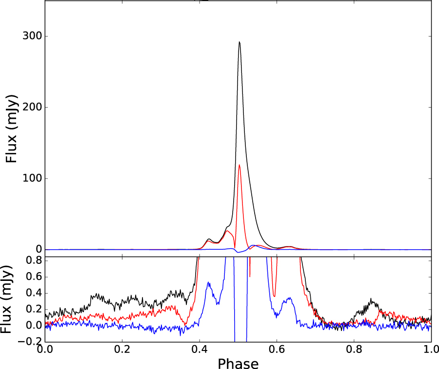
We present the polarization pulse profiles for 28 pulsars observed with the Arecibo Observatory as part of the North American Nanohertz Observatory for Gravitational Waves (NANOGrav) 11-year data set. The high sensitivity of our observations have allowed us to detect low-intensity "microcomponents" in our data set, which can impact the timing of our pulsars and determination of the flux density, as well as give insights into the geometry of the pulsar beam. We were able to describe the time variability of the instrumentation at Arecibo, which when corrected for in the future, will allow us to improve the sensitivity of our gravitational-wave measurements.