The NANOGrav 11-year Data Set: Pulse Profile Variability
by the NANOGrav Collaboration; corresponding author: Paul R. Brook.
Published in The Astrophysical Journal, December 1, 2018.
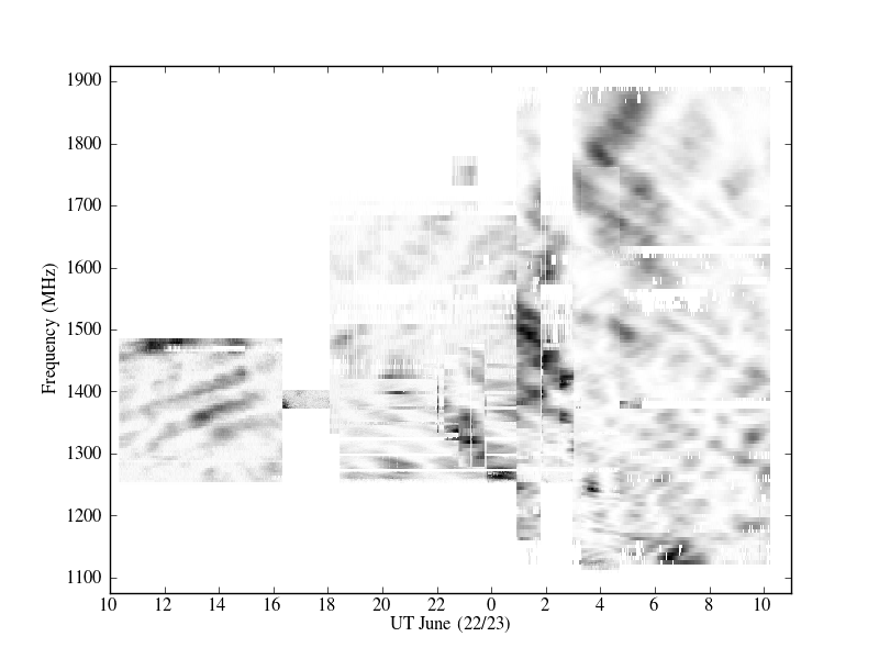
In pulsar timing, we generally assume that the average shape of pulse profiles is stable over the timescale of decades; that is, that if we observe many pulses averaged together from one observation to the next, that they are intrinsically similar. We examined the pulse profiles from the North American Nanohertz Observatory for Gravitational Waves (NANOGrav) 11-year data set to test this assumption and see how they might vary in time. Most of our pulsars show stable profiles though a few do show changes, likely due to the effects of the interstellar medium as the pulses propagate through or due to imperfect polarization calibration. We were able to quantify how variable the pulse profiles were in our data set. Changes in pulse profile changes are detrimental to the accuracy of pulsar timing and must be incorporated into the timing models in the future.