An Acoustical Analogue of a Galactic-scale Gravitational-Wave Detector
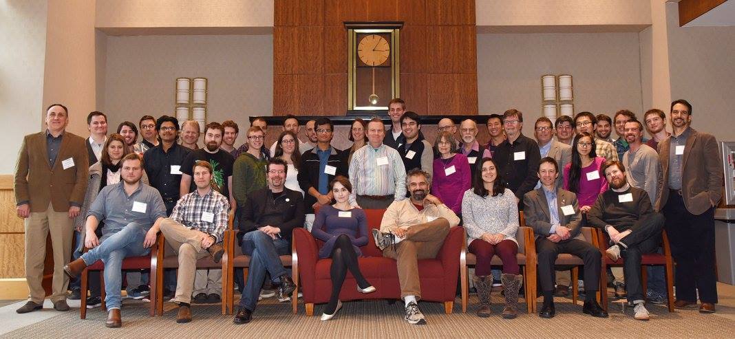
by the NANOGrav Collaboration; corresponding author: Michael T. Lam.
Published in the American Journal of Physics, September 9th, 2018.
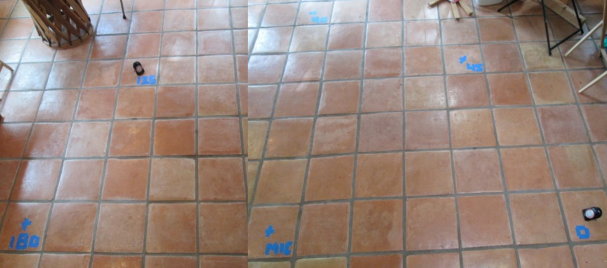
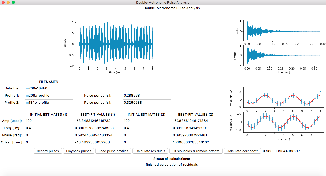
Using a simple microphone and a pair of metronomes, we describe a simple demonstration to illustrate the techniques we use to search for low-frequency gravitational waves. The code we use is available online and an adapted version of the demonstration could be used as an instructional laboratory investigation at the undergraduate or late high school level.