The NANOGrav 11-year Data Set: High-precision Timing of 45 Millisecond Pulsars
by the NANOGrav Collaboration; corresponding author: David J. Nice.
Published in The Astrophysical Journal Supplement Series, April 9th, 2018.
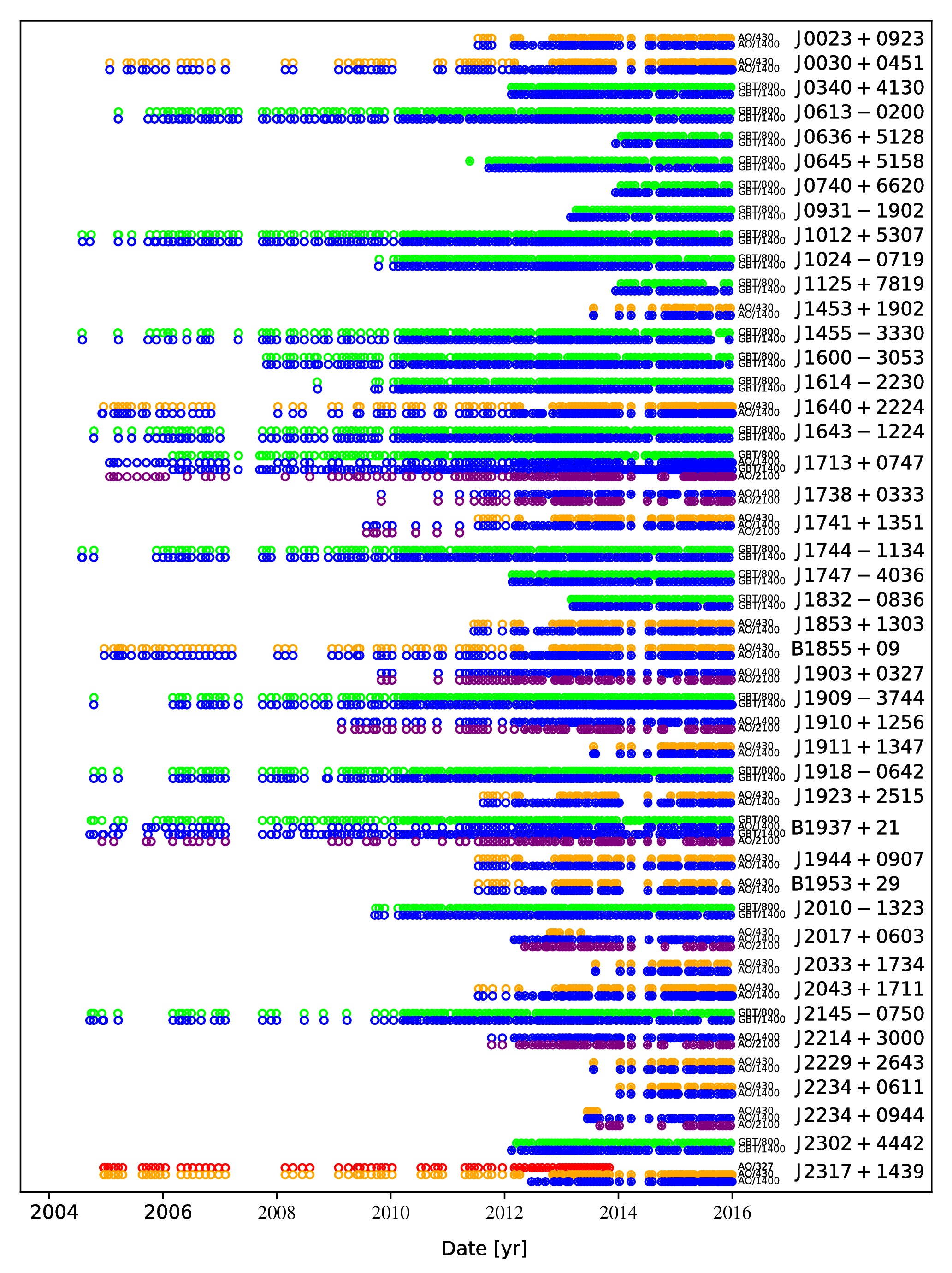
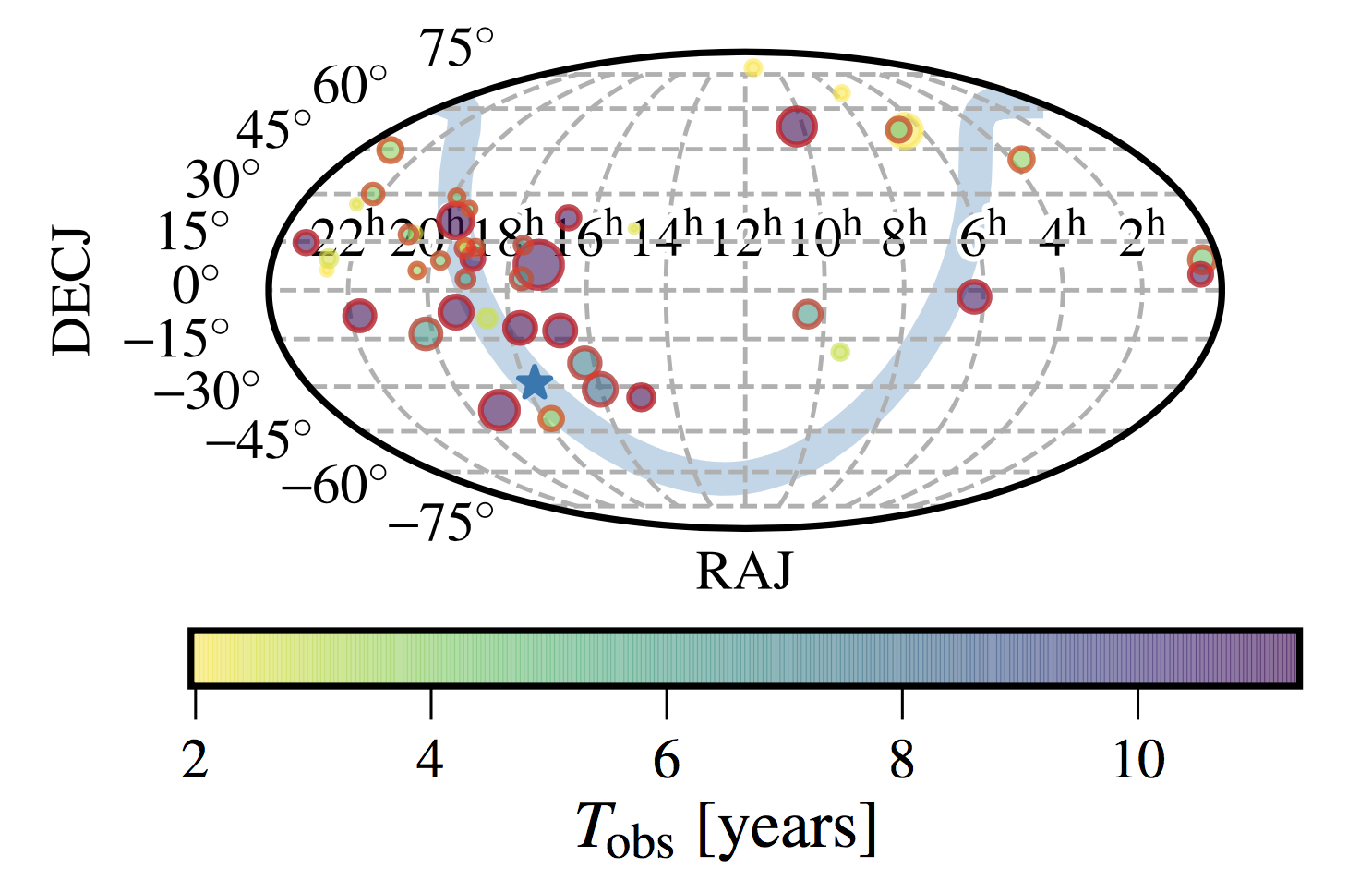
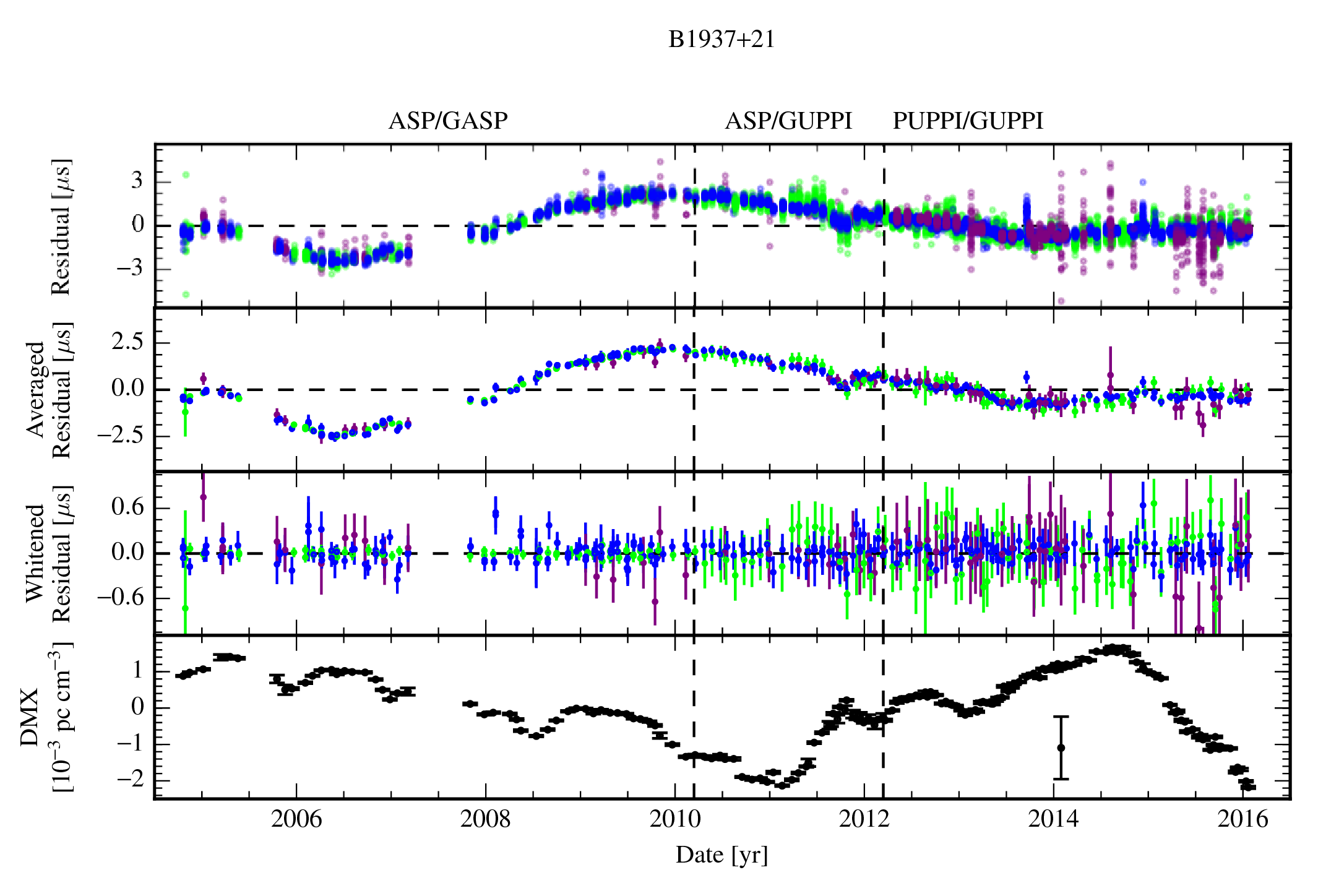
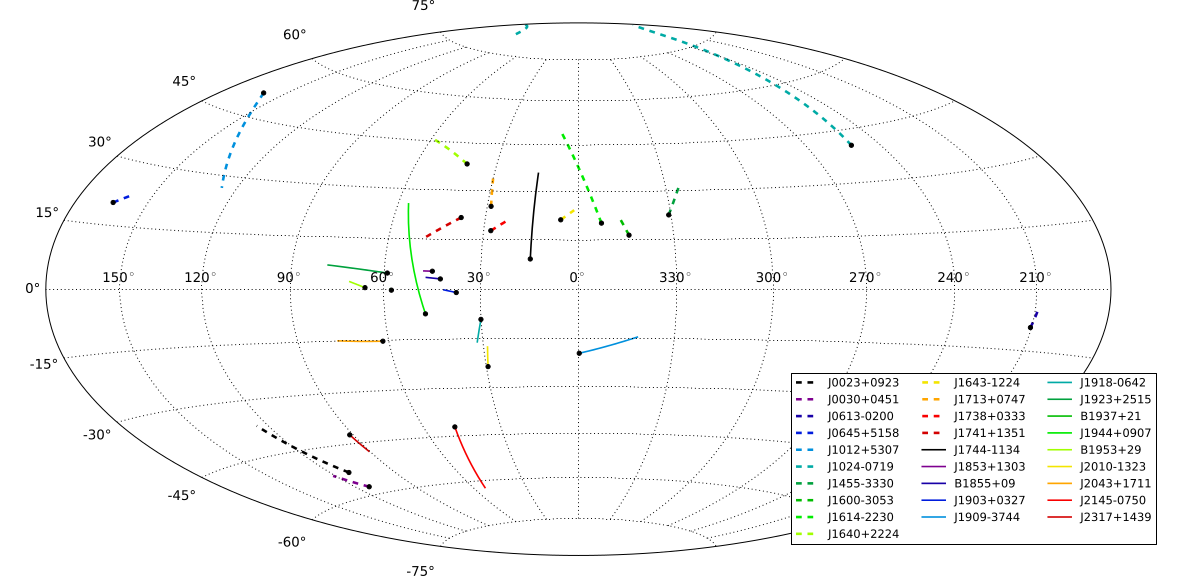
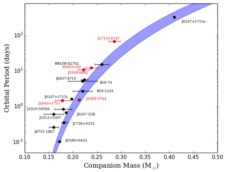
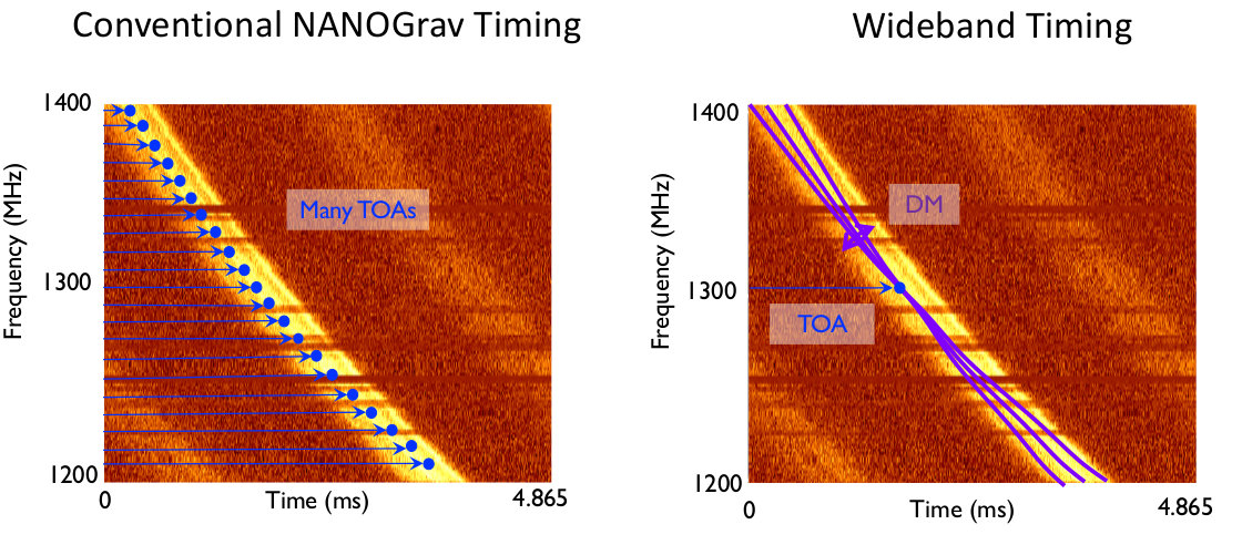
We report on our high-precision timing of 45 millisecond pulsars in the third data set from the North American Nanohertz Observatory for Gravitational Waves (NANOGrav). In addition to providing the timing solutions for these pulsars, we introduce some new techniques in the timing, and discuss new astrometric and binary companion results. This data set has already been used in some of the most stringent constraints on the stochastic gravitational-wave background.